Code
library(ggplot2)
library(dplyr)
library(sf)
library(leaflet)
library(DT)
library(tidyr)
library(htmlwidgets)
library(geeLite)Folks from World Bank data group published a R package that helps to run local R analysis via Google Earth Engine. I’ve already made a demo repository on Github. I think it’s very neat concept that it’s worth spreading.
For this demo, I’ve used:
Install the packages with dependencies. Make sure to use Conda python environment.
library(ggplot2)
library(dplyr)
library(sf)
library(leaflet)
library(DT)
library(tidyr)
library(htmlwidgets)
library(geeLite)In a typical geeLite workflow, you config an R file and download the SQLite DB via GEE API. SQLite database created by the geeLite package. This dataset includes both NDVI (vegetation health) and PTC (tree cover) measurements across hexagonal grid cells covering Turkey.
This section transforms the spatial data into formats suitable for time series analysis and visualization. We extract date columns, reshape the data from wide to long format, and calculate summary statistics for each time period including mean, median, and variability measures across all hexagonal grid cells.
# Load geeLite database with proper path
db <- read_db(path = "data/tr-geelite", freq = "year")

# Load spatial data directly from geeLite database
sf_data <- merge(db$grid, db$`MODIS/061/MOD44B/Percent_Tree_Cover/mean`, by = "id")# Create a function to generate maps for different time periods
create_tree_map <- function(selected_date, data = sf_data, cols = date_cols) {
tree_values <- data[[selected_date]]
valid_tree <- tree_values[!is.na(tree_values)]
# Create color palette with explicit domain range
pal <- colorNumeric("viridis", domain = range(valid_tree, na.rm = TRUE))
# Create leaflet map following blog example
leaflet(data) %>%
addTiles() %>%
addPolygons(
fillColor = ~pal(tree_values),
weight = 1,
color = "#333333",
fillOpacity = 0.9,
popup = ~paste("Percent_Tree_Cover:", round(tree_values, 1),
"<br>Date:", selected_date,
"<br>Hex ID:", id)
) %>%
addScaleBar() %>%
addLegend(
pal = pal,
values = ~tree_values,
title = paste("Percent_Tree_Cover", selected_date),
na.label = "No data",
position = "bottomright"
)
}
# Create maps for several key time periods
sample_dates <- c("2020-01-01", "2021-01-01", "2022-01-01", "2023-01-01", "2024-01-01")
available_dates <- intersect(sample_dates, date_cols)Temporal trends in tree cover across Turkey through two complementary visualizations. The first plot shows the overall trajectory of mean tree cover values, while the second plot illustrates variability and uncertainty by displaying confidence bands around the mean trend along with median values for comparison.
# Time series plot of mean tree cover values
p1 <- ggplot(tree_summary, aes(x = date, y = mean_tree)) +
  geom_line(color = "darkgreen", linewidth = 1.2) +
  geom_point(color = "darkgreen", size = 2) +
  labs(
    title = "Turkey Tree Cover Time Series Analysis (2020-2024)",
    subtitle = "Based on MODIS Tree Cover Data via geeLite",
    x = "Date",
    y = "Mean Tree Cover (%)",
    caption = "Data source: Google Earth Engine via geeLite"
  ) +
  theme_minimal() +
  theme(
    plot.background = element_rect(fill = "#d9d1ba", color = NA),
    panel.background = element_rect(fill = "#d9d1ba", color = NA),
    plot.title = element_text(size = 16, face = "bold", color = "#346b84"),
    plot.subtitle = element_text(size = 12, color = "#346b84"),
    axis.title = element_text(size = 12, color = "#1a3657"),
    axis.text = element_text(size = 10, color = "#1a3657"),
    axis.text.x = element_text(angle = 45, hjust = 1, color = "#1a3657"),
    plot.caption = element_text(color = "#1a3657")
  )

print(p1)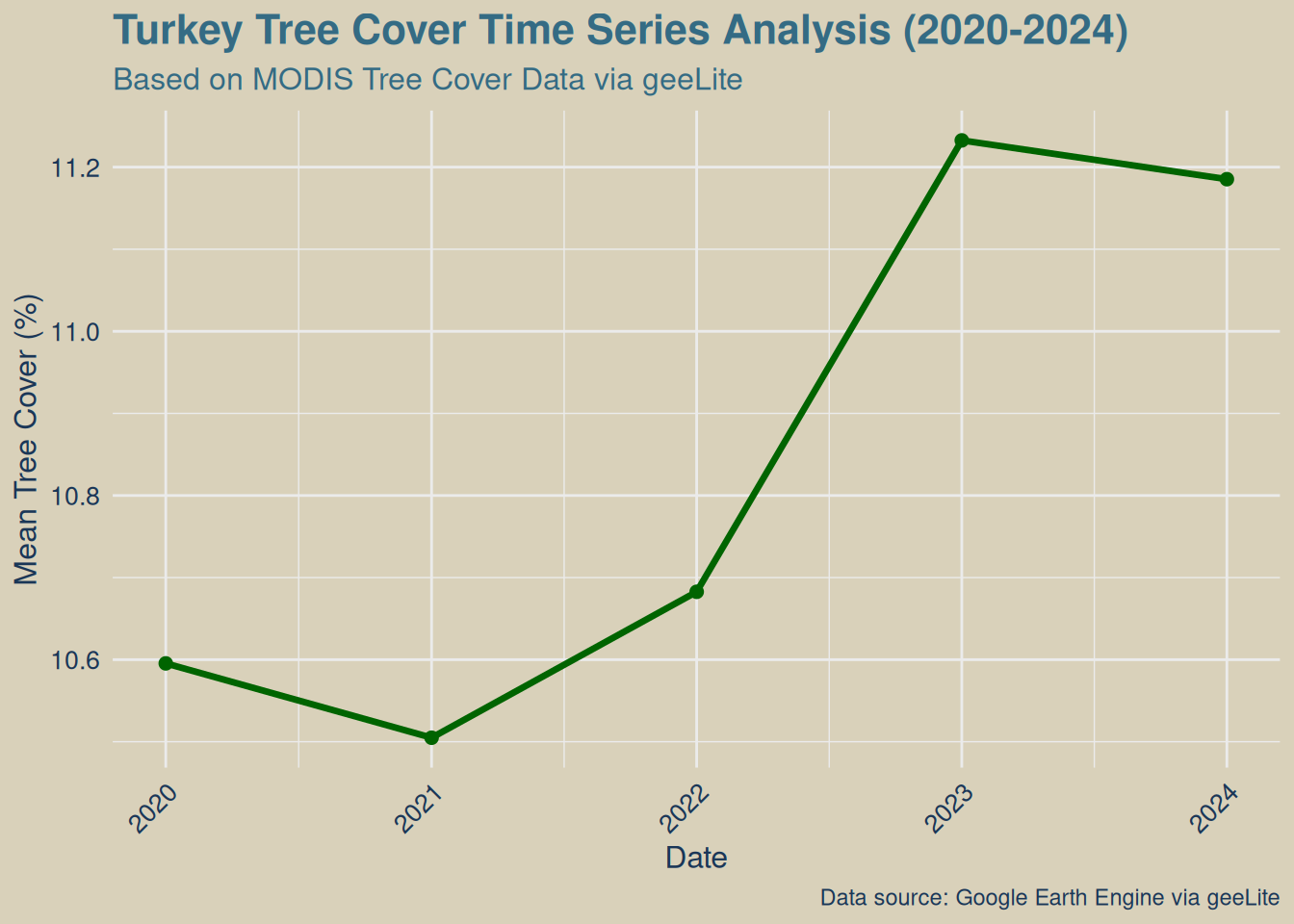
# Plot showing tree cover variability over time
p2 <- ggplot(tree_summary, aes(x = date)) +
  geom_ribbon(aes(ymin = mean_tree - std_tree, ymax = mean_tree + std_tree),
              alpha = 0.3, fill = "green") +
  geom_line(aes(y = mean_tree), color = "darkgreen", linewidth = 1.2) +
  geom_line(aes(y = median_tree), color = "blue", linewidth = 1, linetype = "dashed") +
  labs(
    title = "Tree Cover Variability Across Turkey",
    subtitle = "Mean ± Standard Deviation (green band) and Median (blue dashed)",
    x = "Date",
    y = "Tree Cover (%)",
    caption = "Data source: Google Earth Engine via geeLite"
  ) +
  theme_minimal() +
  theme(
    plot.background = element_rect(fill = "#d9d1ba", color = NA),
    panel.background = element_rect(fill = "#d9d1ba", color = NA),
    plot.title = element_text(size = 16, face = "bold", color = "#346b84"),
    plot.subtitle = element_text(size = 12, color = "#346b84"),
    axis.title = element_text(size = 12, color = "#1a3657"),
    axis.text = element_text(size = 10, color = "#1a3657"),
    axis.text.x = element_text(angle = 45, hjust = 1, color = "#1a3657"),
    plot.caption = element_text(color = "#1a3657")
  )

print(p2)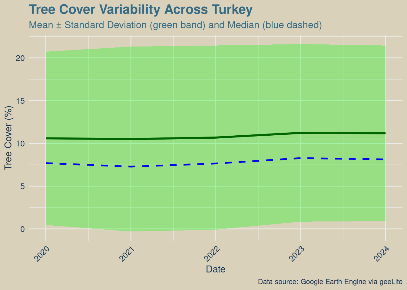
Statistical summaries of the tree cover analysis, including key metrics about data coverage, temporal scope, and overall forest trends. The summary table presents essential findings in a structured format for easy interpretation.
# Calculate overall statistics
baseline_tree <- tree_summary$mean_tree[1]
latest_tree <- tail(tree_summary$mean_tree, 1)
total_change <- latest_tree - baseline_tree
mean_change_per_period <- mean(diff(tree_summary$mean_tree), na.rm = TRUE)

# Create summary table
summary_stats <- data.frame(
  Metric = c("Analysis Period", "Total Observations", "Hexagonal Cells",
             "Baseline Tree Cover", "Latest Tree Cover", "Total Change",
             "Average Change per Period", "Overall Trend"),
  Value = c(
    paste(min(tree_summary$date), "to", max(tree_summary$date)),
    format(nrow(sf_long), big.mark = ","),
    nrow(sf_data),
    paste(round(baseline_tree, 1), "%"),
    paste(round(latest_tree, 1), "%"),
    paste(round(total_change, 1), "%"),
    paste(round(mean_change_per_period, 2), "%"),
    ifelse(total_change > 2, "Forest Improvement",
           ifelse(total_change < -2, "Forest Decline", "Stable"))
  )
)

# Display summary table
knitr::kable(summary_stats,
             caption = "Turkey Tree Cover Analysis Summary",
col.names = c("Metric", "Value"))| Metric | Value |
|---|---|
| Analysis Period | 2020-01-01 to 2024-01-01 |
| Total Observations | 290 |
| Hexagonal Cells | 58 |
| Baseline Tree Cover | 10.6 % |
| Latest Tree Cover | 11.2 % |
| Total Change | 0.6 % |
| Average Change per Period | 0.15 % |
| Overall Trend | Stable |
The interactive table below allows detailed exploration of the time series data. Users can search, sort, and filter the annual tree cover statistics to identify specific patterns or periods of interest. The table includes statistical measures for each time period across all hexagonal grid cells.
# Create interactive data table
DT::datatable(
  tree_summary %>%
    mutate(
      Date = format(date, "%Y-%m-%d"),
      `Mean Tree Cover` = round(mean_tree, 1),
      `Median Tree Cover` = round(median_tree, 1),
      `Min Tree Cover` = round(min_tree, 1),
      `Max Tree Cover` = round(max_tree, 1),
      `Std Dev` = round(std_tree, 1),
      `Valid Cells` = valid_cells
    ) %>%
    select(-date, -mean_tree, -median_tree, -min_tree, -max_tree, -std_tree, -valid_cells),
  caption = "Turkey Tree Cover Time Series Data",
  options = list(
    pageLength = 15,
    scrollX = TRUE,
    dom = 'Bfrtip'
  ),
  rownames = FALSE
)The following table summarizes the key quantitative findings from our analysis, including data coverage metrics, temporal scope, tree cover value ranges, and overall forest change assessment based on the comparison between baseline and latest observations.
# Create results summary data frame
baseline_tree <- tree_summary$mean_tree[1]
latest_tree <- tail(tree_summary$mean_tree, 1)
total_change <- latest_tree - baseline_tree

results_summary <- data.frame(
  Metric = c("Data Coverage", "Time Period", "Tree Cover Range", "Baseline Tree Cover",
             "Latest Tree Cover", "Total Change", "Assessment"),
  Value = c(
    paste(nrow(sf_data), "hexagonal cells across Turkey"),
    paste(length(date_cols), "annual observations from", min(date_cols), "to", max(date_cols)),
    paste(round(min(sf_long$Percent_Tree_Cover, na.rm = TRUE), 1), "% to", round(max(sf_long$Percent_Tree_Cover, na.rm = TRUE), 1), "%"),
    paste(round(baseline_tree, 1), "% (", min(date_cols), ")"),
    paste(round(latest_tree, 1), "% (", max(date_cols), ")"),
    paste(round(total_change, 1), "percentage points"),
    case_when(
      total_change > 2 ~ "FOREST IMPROVEMENT DETECTED 🌱",
      total_change < -2 ~ "FOREST DECLINE DETECTED ⚠️",
      TRUE ~ "Forest cover appears stable"
    )
  )
)

knitr::kable(results_summary, col.names = c("**Metric**", "**Value**"))| Metric | Value |
|---|---|
| Data Coverage | 58 hexagonal cells across Turkey |
| Time Period | 5 annual observations from 2020-01-01 to 2024-01-01 |
| Tree Cover Range | 0.5 % to 44.9 % |
| Baseline Tree Cover | 10.6 % ( 2020-01-01 ) |
| Latest Tree Cover | 11.2 % ( 2024-01-01 ) |
| Total Change | 0.6 percentage points |
| Assessment | Forest cover appears stable |
World Bank Data Team. (2024). geeLite – an R package for tracking remote sensing data locally. World Bank Blogs - Open Data. Available at: https://blogs.worldbank.org/en/opendata/geelite–an-r-package-for-tracking-remote-sensing-datalocally-
Braaten, J., Bullock, E., & Gorelick, N. (2024). geeLite: Client for Accessing and Processing Google Earth Engine Data. GitHub Repository. Available at: https://github.com/gee-community/geeLite
Google Earth Engine Team. (2024). MODIS/061/MOD13A2: MODIS Terra Vegetation Indices 16-Day Global 1km. Google Earth Engine Data Catalog. Available at: https://developers.google.com/earth-engine/datasets/catalog/MODIS_061_MOD13A2